Direct Access
GRACC runs on Elasticsearch, which can be accessed via many client libraries and tools.
A read-only endpoint into the GRACC Elasticsearch is available at https://gracc.opensciencegrid.org/q.
cURL
The Elasticsearch query DSL is quite complex, but is also very powerful. Below is a relatively simple but non-trivial example of directly querying GRACC from the command-line via cURL. This query will calculate the number of payload jobs run by LIGO in January 2017, and the total wall time they used.
curl --header 'Content-Type: application/json' 'https://gracc.opensciencegrid.org/q/gracc.osg.summary/_search?pretty' --data-binary '
{
    "query": {
        "query_string": {
            "query": "VOName:ligo AND ResourceType:Payload AND EndTime:[2017-01-01 TO 2017-02-01]"
        }
    },
    "aggs": {
        "walltime": {
            "sum": {
                "field": "CoreHours"
            }
        },
        "jobs": {
            "sum": {
                "field": "Njobs"
            }
        }
    },
    "size": 0
}'
Which might return:
{
  "took" : 2,
  "timed_out" : false,
  "_shards" : {
    "total" : 6,
    "successful" : 6,
    "failed" : 0
  },
  "hits" : {
    "total" : 68,
    "max_score" : 0.0,
    "hits" : [ ]
  },
  "aggregations" : {
    "jobs" : {
      "value" : 20626.0
    },
    "walltime" : {
      "value" : 41323.43916666666
    }
  }
}
Compare to the VO Summary dashboard in Grafana.
Python (elasticsearch-dsl)
In this example we use the elasticsearch-dsl package to query the cumulative
walltime and cpu time for some selected VOs for the past 90 day.
We'll then calculate the CPU efficiency for each.
We'll then load the results into a pandas dataframe for further analysis and plotting with matplotlib.
Query Elasticsearch
from elasticsearch import Elasticsearch
gracc=Elasticsearch('https://gracc.opensciencegrid.org/q',timeout=120)
from elasticsearch_dsl import Search

# All FIFE VOs running on GPGrid
q='ProbeName:*fifebatch* AND Host_description:GPGrid'
# Last 90 days
start='now-90d'
end='now'
# GRACC summary index
i='gracc.osg.summary'

s = Search(using=gracc, index=i) \
    .filter("range",EndTime={'gte':start,'lte':end}) \
    .query("query_string", query=q)

s.aggs.bucket('vo', 'terms', field='VOName', size=20, order={'WallHours':'desc'}) \
    .metric('WallHours', 'sum', field='CoreHours') \
    .metric('UserCpuSeconds', 'sum', field='CpuDuration_user') \
    .metric('SysCpuSeconds', 'sum', field='CpuDuration_system')

#print s.to_dict()
r = s.execute()
Print buckets
for vo in r.aggregations.vo.buckets:
    eff = (vo.UserCpuSeconds.value+vo.SysCpuSeconds.value)/vo.WallHours.value/3600.0*100.0
    print '%20s\t%10.0f\t%5.2f%%' % (vo.key, vo.WallHours.value, eff)
                nova       6144687  61.32%
               minos       4332035  92.74%
                mu2e       4143032  87.56%
          microboone       3085974  68.13%
             minerva       2600511  62.41%
                mars       2030271  84.34%
                dune       1576534  82.17%
                 des       1523825  40.31%
            seaquest        944561  69.49%
                 cdf        722131  72.49%
                 gm2        621704  75.38%
            darkside        533901  41.15%
              lariat        256586  46.81%
               annie        137215  53.45%
                cdms         88995  85.85%
                sbnd         84224  76.48%
            argoneut          9975  85.41%
            fermilab          8294  95.52%
               genie          3386  72.48%
               coupp          2834  20.46%
Pull aggregation results into pandas
from pandas.io.json import json_normalize
#df = json_normalize(r.aggs.vo.buckets.__dict__['_l_'])
df = json_normalize(r.to_dict()['aggregations']['vo']['buckets'])
df.head()
| SysCpuSeconds.value | UserCpuSeconds.value | WallHours.value | doc_count | key | |
|---|---|---|---|---|---|
| 0 | 51333597.0 | 1.350929e+10 | 6.140375e+06 | 2868 | nova |
| 1 | 30771554.0 | 1.435938e+10 | 4.311367e+06 | 746 | minos |
| 2 | 111866383.0 | 1.294148e+10 | 4.140957e+06 | 1002 | mu2e |
| 3 | 313454481.0 | 7.251906e+09 | 3.080024e+06 | 3355 | microboone |
| 4 | 37939287.0 | 5.800780e+09 | 2.599362e+06 | 1734 | minerva |
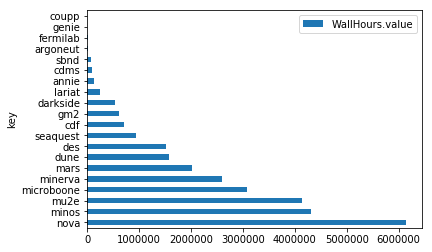
%matplotlib inline

df.plot.barh(x='key',y='WallHours.value')
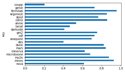
Calculate efficiency
def efficiency(row):
    return (row['UserCpuSeconds.value']+row['SysCpuSeconds.value'])/row['WallHours.value']/3600.0
df['efficiency']=df.apply(efficiency,axis=1)
df.plot.barh(x='key',y='efficiency',legend=False)